I clipped it carelessly but I’m quite happy with it given I’ve never mixed DnB before about 2pm today 😀
Hope someone enjoys 🙂
I clipped it carelessly but I’m quite happy with it given I’ve never mixed DnB before about 2pm today 😀
Hope someone enjoys 🙂
This is something I spent a lot of time working on for Oxford Wave Research’s SpectrumView app.
I saw a question on stackoverflow today on exactly all the problems I spent a good while working out over time so I thought I’d share my response on my blog for posterity. It now follows:
Well it all depends on the frequency range you’re after. An FFT works by taking 2^n samples and providing you with 2^(n-1) real and imaginary numbers. I have to admit I’m quite hazy on what exactly these values represent (I’ve got a friend who has promised to go through it all with me in lieu of a loan I made him when he had financial issues ;)) other than an angle around a circle. Effectively they provide you with an arccos of the angle parameter for a sine and cosine for each frequency bin from which the original 2^n samples can be, perfectly, reconstructed.
Anyway this has the huge advantage that you can calculate magnitude by taking the euclidean distance of the real and imaginary parts (sqrtf( (real * real) + (imag * imag) )). This provides you with an unnormalised distance value. This value can then be used to build a magnitude for each frequency band.
So lets take an order 10 FFT (2^10). You input 1024 samples. You FFT those samples and you get 512 imaginary and real values back (the particular ordering of those values depends on the FFT algorithm you use). So this means that for a 44.1Khz audio file each bin represents 44100/512 Hz or ~86Hz per bin.
One thing that should stand out from this is that if you use more samples (from whats called the time or spatial domain when dealing with multi dimensional signals such as images) you get better frequency representation (in whats called the frequency domain). However you sacrifice one for the other. This is just the way things go and you will have to live with it.
Basically you will need to tune the frequency bins and time/spatial resolution to get the data you require.
First a bit of nomenclature, the 1024 time domain samples I referred to earlier is called your window. Generally when performing this sort of process you will want to slide the window on by some amount to get the next 1024 samples you FFT. The obvious thing to do would be to take samples 0->1023, then 1024->2047, and so forth. This unfortunately doesn’t give the best results. Ideally you want to overlap the windows to some degree so that you get a smoother frequency change over time. Most commonly people slide the window on by half a window size. ie your first window will be 0->1023 the second 512->1535 and so on and so forth.
Now this then brings up one further problem. While this information provides for perfect inverse FFT signal reconstruction it leaves you with a problem that frequencies leak into surround bins to some extent. To solve this issue some mathematicians (far more intelligent than me) came up with the concept of a window function. The window function provides for far better frequency isolation in the frequency domain though leads to a loss of information in the time domain (ie its impossible to perfectly re-construct the signal after you have used a window function, AFAIK).
Now there are various types of window function ranging from the rectangular window (effectively doing nothing to the signal) to various functions that provide far better frequency isolation (though some may also kill surrounding frequencies that may be of interest to you!!). There is, alas, no one size fits all but I’m a big fan (for spectrograms) of the blackmann-harris window function. I think it gives the best looking results!
However as I mentioned earlier the FFT provides you with an unnormalised spectrum. To normalise the spectrum (after the euclidean distance calculation) you need to divide all the values by a normalisation factor (I go into more detail here).
this normalisation will provide you with a value between 0 and 1. So you could easily multiple this value by 100 to get your 0 to 100 scale.
This, however, is not where it ends. The spectrum you get from this is rather unsatisfying. This is because you are looking at the magnitude using a linear scale. Unfortunately the human ear hears using a logarithmic scale. This rather causes issues with how a spectrogram/spectrum looks.
To get round this you need to convert these 0 to 1 values (I’ll call it ‘x’) to the decibel scale. The standard transformation is 20.0f * log10f( x ). This will then provide you a value whereby 1 has converted to 0 and 0 has converted to -infinity. your magnitudes are now in the appropriate logarithmic scale. However its not always that helpful.
At this point you need to look into the original sample bit depth. At 16-bit sampling you get a value that is between 32767 and -32768. This means your dynamic range is fabsf( 20.0f * log10f( 1.0f / 65536.0f ) ) or ~96.33dB. So now we have this value.
Take the values we’ve got from the dB calculation above. Add this 96.33 value to it. Obviously the maximum amplitude (0) is now 96.33. Now didivde by that same value and you nowhave a value ranging from -infinity to 1.0f. Clamp the lower end to 0 and you now have a range from 0 to 1 and multiply that by 100 and you have your final 0 to 100 range.
And that is much more of a monster post than I had originally intended but should give you a good grounding in how to generate a good spectrum/spectrogram for an input signal.
and breathe
As an aside I found kiss FFT far easier to use, my code to perform a forward fft is as follows:
    CFFT::CFFT( unsigned int fftOrder ) :
        BaseFFT( fftOrder )
    {
    	mFFTSetupFwd	= kiss_fftr_alloc( 1 << fftOrder, 0, NULL, NULL );
    }

    bool CFFT::ForwardFFT( std::complex< float >* pOut, const float* pIn, unsigned int num )
    {
    	kiss_fftr( mFFTSetupFwd, pIn, (kiss_fft_cpx*)pOut );
    	return true;
    }
So its been a while since I posted anything up here *cough*.
Over the past year things have gone a bit strange. As a result I have no left my former employer and am going into business with the chap who was my boss.
We will now be available for contract work.
Primarily we are both very experienced on statistical analysis of audio streams (For acoustic event recognition for one) and would like to do a lot more more research in this area. We will also be looking to extend our research capabilities into video as I have a fair bit of experience at dealing with 2D signals (ie Video).
On top of that we will also be available for contract app development for PC, Mac, Linux, iPhone, Android and Windows mobile 7.
Anyone who wants more information about my skills should check my linkedin page at:
http://uk.linkedin.com/pub/oscar-forth/8/857/22
And/Or Anil’s at:
http://uk.linkedin.com/in/anilalexander
Well 2 weeks of trying to fins bugs in a piece of software I’ve written at work only to discover that only the Dell machine was getting the problem.
This morning, thanks to this wonderful blog post from Mark Russinovich we finally tracked the problem to a non-paged pool leak. On closer inspection (ie going through the steps Mark lists) we realised that there was a leak in WavXDocMgr.sys. After much hunting around we discovered that this is in the Dell Control Point Security Manager. We uninstalled it and the leak has gone.
Couple that with the multiple hardware failure we had on this machine and I can honestly say “Cheers Dell”. You’ve caused us to truly f**k off a customer and absorbed waaaay more of my time on one problem than I would have ever thought possible.
The code I’ve already given for doing wavelet transforms is very simple but I treat horizontal and vertical passes as seperate functions. It occurred to me as I looked at those functions that they are, essentially, the same. The only real difference is how many pixels you step over to get to the next or previous one. This was a massive realisation to me. It meant that I could do all my wavelet transforms through a single function.
Here is the Foward transform function:
const int32_t postDwtNum	= dwtMax / 2;

const int32_t nextReadOffset2		= nextReadOffset * 2;
//const int32_t nextWriteOffset2		= nextWriteOffset * 2;

int32_t readOffset	= startOffset;

int32_t s			= readOffset;
int32_t d			= readOffset	+ (postDwtNum * nextWriteOffset);

const DataType d1	= m_SignalData[readOffset + nextReadOffset]	- (((m_SignalData[readOffset]	+ m_SignalData[readOffset + nextReadOffset2])	/ (DataType)2));
const DataType s1	= m_SignalData[readOffset]					+ (((d1							+ d1)											/ (DataType)4));

out.m_SignalData[d]	= d1;
out.m_SignalData[s]	= s1;

s	+= nextWriteOffset;
d	+= nextWriteOffset;

readOffset	+= nextReadOffset2;

int dwt = 2;
while( dwt < dwtMax - 2 )
{
	const DataType d1	= m_SignalData[readOffset + nextReadOffset]	- (((m_SignalData[readOffset]				+ m_SignalData[readOffset + nextReadOffset2])	/ (DataType)2));
	const DataType s1	= m_SignalData[readOffset]					+ (((out.m_SignalData[d - nextWriteOffset]	+ d1)											/ (DataType)4));

	out.m_SignalData[d]	= d1;
	out.m_SignalData[s]	= s1;

	s	+= nextWriteOffset;
	d	+= nextWriteOffset;

	readOffset	+= nextReadOffset2;

	dwt += 2;
}
{
	const DataType d1	= m_SignalData[readOffset + nextReadOffset]	- (((m_SignalData[readOffset]				+ m_SignalData[readOffset])	/ (DataType)2));
	const DataType s1	= m_SignalData[readOffset]					+ (((out.m_SignalData[d - nextWriteOffset]	+ d1)						/ (DataType)4));

	out.m_SignalData[d]	= d1;
	out.m_SignalData[s]	= s1;
}
return true;
What a relisation this was! This meant that I could now generalise the algorith to handle multi dimension signals. A 1D signal is pretty simple and is a single call to this function per wavelet "level"
int32_t level	= 0;
while( level < numLevels )
{
	Signal< DataType >::FDWT( 0, 1, 1, GetWidth() >> level, out );
	level++;
}
A 2D signal is a little more complicated as you need to do it for each horizontal line of an image and then each vertical line of an image. The code however still goes through that one function and looks something like this:
// Now run DWT.
int32_t level	= 0;
while( level < numLevels )
{
	int32_t y		= 0;
	int32_t yMax	= GetHeight() >> level;
	while( y < yMax )
	{
		out.Signal< DataType >::FDWT( y * GetWidth(), 1, 1, GetWidth() >> level, out2 );			// Horizontals
		y++;
	}

	int32_t x		= 0;
	int32_t xMax	= GetWidth() >> level;
	while( x < xMax )
	{
		out2.Signal< DataType >::FDWT( x, GetWidth(), GetWidth(), (GetHeight() >> level), out );	// Verticals
		x++;
	}
	level++;
}
Now this then led me on to thinking about a 3D signal. To do the forward transform a 3D signal would now mean for each depth slice performing the 2D transform as above. After that you would then perform the transform a long a depth line or constant row and column. Thats a hell of a lot of calculations but I "think" (Though I have not tested this at all) that the code would look something like this:
int32_t level	= 0;
while( level < numLevels )
{
	int32_t z		= 0;
	int32_t zMax	= GetDepth();
	while( z < zMax )
	{
		int32_t y		= 0;
		int32_t yMax	= GetHeight();
		while( y < xMax )
		{
			out2.Signal< DataType >::FDWT( (y * GetWidth()) + (z * widthHeight), 1, 1, GetWidth() >> level, out );	// Horizontals
			x++;
		}

		int32_t x		= 0;
		int32_t xMax	= GetWidth();
		while( x < xMax )
		{
			out.Signal< DataType >::FDWT( x, GetWidth(), GetWidth(), GetHeight() >> level, out2 ); // Verticals
			x++;
		}
		z++;
	}

	int32_t y		= 0;
	int32_t yMax	= GetHeight();
	while( y < yMax )
	{
		int32_t x		= 0;
		int32_t xMax	= GetWidth();
		while( x < xMax )
		{
			out2.Signal< DataType >::FDWT( x + (y * GetWidth()), GetWidth() * GetHeight(),  GetWidth() * GetHeight(), GetDepth() >> level, out ); // "Depthicals"
			x++;
		}
		y++;
	}


	level++;
}
This 3D method gives a potential compression schemes for video. Though I'd hate to think the kind of horsepower you'd need to have available to process a video real-time.
Allin, I cannot believe I didn't spot this simplification before hand ...
So it turned out that the refinement pass was actually pretty easy to do.
Lets say I’m compressing a pixel with a value of -129 and I’m using a threshold of 128. I push into a vector the value |129| – 128. ie the absoloute value minus the threshold. I subsequently do this for every pixel above my threshold.
pixelsForRefinement.push_back( absVal - threshold );
I then halve the threshold and do the same sort of processing again. Now I run through the values that were pushed into my vector on the pass before hand and I do a simple check. Is the value in the vector (in the example case 1) greater than 128? No so I write a 0 to the refinement stream. If it IS greater than I write a 1 to the refinement stream and subtract the threshold value from the value stored in the vector.
// We now need to refine the pixels that were added on the previous pass
uint32_t refinement		= 0;
uint32_t refinementMax	= lastNumPixelsForRefinement;
while( refinement < refinementMax )
{
	const int16_t val				= pixelsForRefinement[refinement];
	const BitEncoding::Bit bit		= (val >= threshold) ? BitEncoding::Bit_One : BitEncoding::Bit_Zero;
	pixelsForRefinement[refinement]	-= (threshold * (uint32_t)bit);

	bitStreamOut.refineBitStream	+= bit;

	refinement++;
}
lastNumPixelsForRefinement	= pixelsForRefinement.size();
Effectively this means that for each pass through I refine the already WDR’d pixels by the current threshold.
The result is a perfect re-construction from the wavelet information (I shan’t bother posting up a before and after picture as they look the same ;)).
Now to get some form of compression I need to be able to early out from the algorithm and, basically, only store high frequency information (as well as the low frequency image in the first place). This posed a slight problem, however as I need to be able to perform the compression on each wavelet step as I go along. The system I had built thus far performed the compression on all the LH etc segments for each wavelet decomposition level. I needed to do some code re-organisation to get it do them in the correct order (ie LH, HL and HH). It wasn’t too difficult.
At this point though I realised I could MASSIVELY simplify the wavelet transforms. This I will explain in the next article.
Its been slightly under a month since my last post. In the interim I have done much battling with a teething baby that has resulted in a lack of motivation to attack a complicated problem. The past couple of nights, though, I have set back to the WDR compressor with the intention of getting it working.
I now, fortunately, have a limited compressor/decompressor going.
In the previous article I described the basics behind a Daub 5/3 forward wavelet transform. In this article I will be describing how to do the significance pass of the WDR algorithm.
The basic idea is to run through the high pass sections of the image (LH, HL and HH) with a specific threshold. At each threshold level the algorithm needs to find the number of pixels to the next pixel that is greater than (or equal to) the threshold.
For example, take an image that has these values stored in its high pass:
0 0 -2 0 0 8 0 0
0 9 0 -3 0 4 0 0
0 0 1 7 0 0 6 0
0 5 0 0 0 -8 0 1
0 0 0 0 0 0 2 0
0 0 -4 0 6 0 0 0
0 3 0 0 0 7 0 0
0 -8 0 0 0 0 5 0
0 0 0 0 -2 0 0 0
First start with an arbitrary threshold. In this example I will choose 8. We now start from the beginning and scan through for the first value greater-than-or-equal-to 8. Pixel 6 is the first, pixel 10 is the next, pixel 30 the 3rd and so on. In WDR we want the difference between those pixels. So We would store 6, 4 and 20 for the 3 pixels above. The other obvious part is the sign. In fact we’d want to store those first 3 pixels as +6, +4 and -20. When you have found all the pixels in the image that are above your threshold then you write a + to indicate the end of a run (Though I’m pretty sure it would be quite simple to eliminate the trailing +). You then halve the threshold and process again (Though ignoring the pixels you have already processed).
Thats the basics. Of course its far more complicated than that. For one each high pass section of the image is read in a different way and not as simply as I explained above. This is explained in many papers on WDR (An example). The scan orders are as follows:
For LH:
1 2 3 4
8 7 6 5
9 10 11 12
16 15 14 13
(ie You go form left to right on odd lines and right to left on even forming a weaving pattern)
For HL:
1 8 9 16
2 7 10 15
3 6 11 14
4 5 12 13
(ie Similar to LH but vertical scans instead of horizontal)
For HH:
1 2 6 7
3 5 8 13
4 9 12 14
10 11 15 16
(ie This one is performed by zig-zagging across the texture).
The reason the image is processed in this way is to try and maximise the runs of pixels that you will get. Again this is all explained well in various papers (Though it may well be interesting to play with these to see if you get better compressions by running across the pixels in different ways).
So now you have your list of differences and signs for a set of thresholds. The final part of the WDR algorithm is to bit encode your data. This is something that is poorly explained in many of the articles that I have read, I would truly have been lost if it was not this paper. If we look at the bit patterns of each of the numbers we retrieved earlier (ie 6 = 110, 4 = 100 and 20 = 10100) we can see that the highest bit is always 1 this is the case for all our numbers (If this doesn’t seem obvious now scribble out some binary numbers and you will see why its quite obvious!). Thus when bit encoding we can ignore the leading 1 and store the subsequent bits (ie 10, 00, 0100). Brilliant. We do, however, need to store the sign along side this number. For this reason we use a 2 bit per digit scheme. – = 11, + = 10, 1 = 01, 0 = 00. Armed with this information we can store the numbers in a bit stream as 100100 — 100000 — 11000100. When we build this up over each pass for each threshold we end up saving quite a few bits. This is the main meat of the compression.
Of course writing the bits is not the most fun of things. For this reason I wrote my own templated bitstream class for handling easy addition and lookup of the bit patterns I was after.
My code looked something like this:
 int count	= 0;
int max	 = (width >> 1) * (height >> 1);
while( count < max ) { const int pixelStart	= buffStart	+ iter->GetX() + (iter->GetY() * pitch);
const int16_t val	 = plane.pixels[pixelStart];
const int16_t absVal	= abs( val );
if ( absVal > threshold && absVal < (threshold << 1))
{
	// Push sign.
	bitStreamOut.wdrBitStream += (val < 0) ? BitEncoding::Bit_Minus : BitEncoding::Bit_Plus;
	// Push numbers into bit stream.
	uint8_t bitNum	 = 0;//HighestBitSet( pixelPos );;
	uint8_t bitMax	 = HighestBitSet( pixelPos );
	while( bitNum < bitMax )
	{
		bitStreamOut.wdrBitStream	+= (((pixelPos & (1 << bitNum)) >> bitNum) == 0) ? BitEncoding::Bit_Zero : BitEncoding::Bit_One;
		bitNum++;
	}
	pixelPos	= 1;
}
pixelPos++;
iter->Next();
count++;
}
//Emit +remainingPixels+ to indicate end …
bitStreamOut.wdrBitStream += BitEncoding::Bit_Plus;
uint8_t bitNum	 = 0;//HighestBitSet( pixelPos );;
uint8_t bitMax	 = HighestBitSet( pixelPos );
while( bitNum < bitMax )
{
	bitStreamOut.wdrBitStream	+= (((pixelPos & (1 << bitNum)) >> bitNum) == 0) ? BitEncoding::Bit_Zero : BitEncoding::Bit_One;
	bitNum++;
}
bitStreamOut.wdrBitStream += BitEncoding::Bit_Plus;
Something to note in the code ismy iter->Next() which is one of my 3 iterators that define the way we wind through each highpass section.
We now have a compressed bit stream. I used the now ubiquitous lena image for testing this out.
This is the result of the Wavelet transform:

The arrangement of this image is slightly backward. This is due to the way windows reverses images. You can however see the HL and HH passes on the top and the LL and LH passes on the bottom (instead of the other way round).
From there we need to decompress the bit stream and end up with something like the original image:

This decompression took me a while to get right. Basically, though, you need to go back over the bit stream dropping the appropriate bits in the correct places until you get back an image like the former. Running the inverse wavelet transform should result in the above image.
Easy for me to say. Firstly we need to drop the correct values in the correct places. To do this we need the original threshold value we started with. The bit stream will always start with a plus or minus. Following that we have the bits of the difference value. When we find another sign we are on to the next pixel. Don’t forget that the 1 needs to be added to the left of the number! When we get a number that takes us to the end of the image we will find an extra plus and we can go back to the beginning at half the threshold.
So the first value we get out is a 6 and we have a sign of +. This means we are writing a +8 at the 6th pixel position. We then read a +4 so we are writing a +8 at the 10th position. We next get that -20 which means we write a -8 at the 30th position and so on.
The quick (er than me) will noticed that this means that the value of 9 in our earlier example will get written back as an 8 (or a value of 7 written as a 4). This is where the refinement pass comes in. I will explain this in a further article (ie when I get it working ).
My code for doing this looked something like the following:
iter->SetToStart();

int pixelPos                = 0;
while( pixelPos < size )
{
	int sign                    = bitStream.wdrBitStream[bit];
	bit++;

	int pixelDiff               = 0;
	int bitPos                  = 0;
	BitEncoding::Bit readBit    = BitEncoding::Bit_Zero;
	while( readBit < BitEncoding::Bit_Plus )
	{
		readBit = bitStream.wdrBitStream[bit];
		switch( readBit )
		{
		case BitEncoding::Bit_One:
			pixelDiff   |= readBit << bitPos;
		case BitEncoding::Bit_Zero:
			bitPos++;
			break;

		case BitEncoding::Bit_Minus:
		case BitEncoding::Bit_Plus:
			break;

		}
		bit++;
	}
	pixelDiff   |= 1 << bitPos;   // Always a 1 at the top end.

	pixelPos    += (pixelDiff - 1);

	if ( pixelPos < size )
	{
		// Step forward through the iterator pixelPos times.
		uint32_t count  = 0;
		while( count < pixelDiff )           {               count++;               iter->Next();
		}

		const uint32_t writePos   = buffStart   + (iter->GetX() + iter->GetY() * pitch));
		planeOut.pixels[writePos] = (sign == BitEncoding::Bit_Plus) ? threshold : -threshold;

		bit--;
	}
}
Of course you can run the wavelet transform on the low-pass sub-image created from previous steps. This will give you something like the following:

Decompressing this image returns you to the following:

In this you can see some colour errors. I think this is caused by my lack of a refinement pass however its well worth noting the details on her hat brim and her boa. Both of these have returned and look good in the re-sized image.
Anyway … should anyone actually be reading my ramblings or have any questions then say hi in the comments!
Update: I identified a bug whereby the software would get confused by a 0 and a 1 appearing in the WDR stream as both end up as the same value. Zeros really shouldn’t be turning up so this has now been fixed.
I’ve now spent a few weekends working on my WDR system. The one overriding thing that gets to me is just how bad the information is out there. There are lots of things that aren’t quite spelled out well enough for non-maths gods like me.
Anyway. On to the basics of the transform. Anyone who has dealt with wavelets knows that you decompose the image into 4 sections.
LL LH
HL HH
You then go on to to the same process to the LL portion of the image. Rinse and repeat this method for as long or as short as you like (You don’t have to even do more than the first decomposition). Effectively what you now have is high pass information and low pass information. The low pass is the LL section. The highpass sections give you the horizontal high pass, the vertical high pass and the diagonal high pass (Effectively edge detect in 3 different directions). These are generated by first applying the wavelet transform horizontally and then applying it on the resulting image vertically. The joy of the wavelet transform is that it is reversible. Exactly so. This means you can re-construct the original image from the various high and low passes losslessly. Its worth bearing in mind that this can be trivially extended into 3 dimensions to compress video. I keep wondering whether you’d be able to re-sample frame rates nicely using this sort of video transform but thats an aside.
Ok so lets get on to a wavelet transform. I’m going to use the Daub5/3 wavelet because it can be done entirely with integers which means there are no rounding issues. It is truly lossless.
The equation is as follows (Taken from: A Low-power, Low-memory System for Wavelet-based Image Compression by Walker, Nguyen & Chen):
My first thought on seeing that was WTF!? However I carried on reading through the excellent paper linked above.
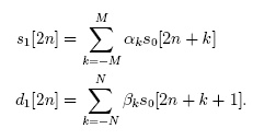
It turns out that there is a more efficient (And simpler) form of this wavelet transform known as a lifting wavelet transform. The transform looks like the following:

First thing to notice is that the calculation for s1 contains usage of d1. Not just d1 but the previous pixel’s d1.
(At this juncture I’d like to point out that the aforementioned paper gives another equation as an “integer-to-integer” equation. Try as I might I could never get this working. The equation I’ve just posted works perfectly).
I’m going to move on to some code now.
const int n = (x) + (y * pixelPitch);
const int n2 = (x / 2) + (y * pixelPitch);
const int s = n2;
const int d = n2 + widthDiv2;
const int16_t d1 = pixelsIn[n + 1] –
(((pixelsIn[n] + pixelsIn[n + 2]) >> 1));
const int16_t s1 = pixelsIn[n] +
(((pixelsOut[d – 1] + d1) >> 2));
pixelsOut[d] = d1;
pixelsOut[s] = s1;
The above is a simple code version of the wavelet transform. There is a problem with it, however. You’ll note that due to the fact it uses the previous high pass pixel outputed in the s1 calculation and the next pixel from the input in the d1 calculation.
This means that we get a break down at either end of a line. Fortunately this is fairly easy to rectify (Though I can find no mention of it anywhere). For the first pixel on a line you can just use d1 twice. For the last pixel you use the current pixel twice. Its an easy solution and works well.
When doing a vertical decomposition the equation is much the same but instead of doing -1, +1 and +2 by adding/subtracing the pixel pitch (The width of the entire original texture) instead of 1. Doing this twice over performs the appropriate 2D forward wavelet transform.
Inverting the wavelet transform is pretty simple as well. You can easily get the reverse of the transform by re-arranging the equations. Bear in mind, however, that you need to step from the right hand side of the image towards the left (ie backwards) to re-construct the image. The trick above for handling the special cases at either end of the line works just as well for the inverse transform.
The code for the central part of the inverse transform will look something like this:
const int n = (x) + (y * pixelPitch);
const int n2 = (x / 2) + (y * pixelPitch);
const int s = n2;
const int d = n2 + widthDiv2;
const int16_t s0 = pixelsIn[s] –
(((pixelsIn[d – 1] + pixelsIn[d]) >> 2));
const int16_t s1 = pixelsIn[d] +
(((s0 + pixelsOut[n + 2]) >> 1));
pixelsOut[n] = s0;
pixelsOut[n + 1] = s1;
Anyway I hope thats slightly useful. It certainly will be to me when I inevitably forget what I’ve done 🙂
I intend this blog to represent my various programming related interests. I have been working on a Daub 5/3 based WDR compression scheme. When I get the chance I will describe how exactly I got this working. However I have re-started my alcohol drinking (post detox) so it may take longer than I intend 😉